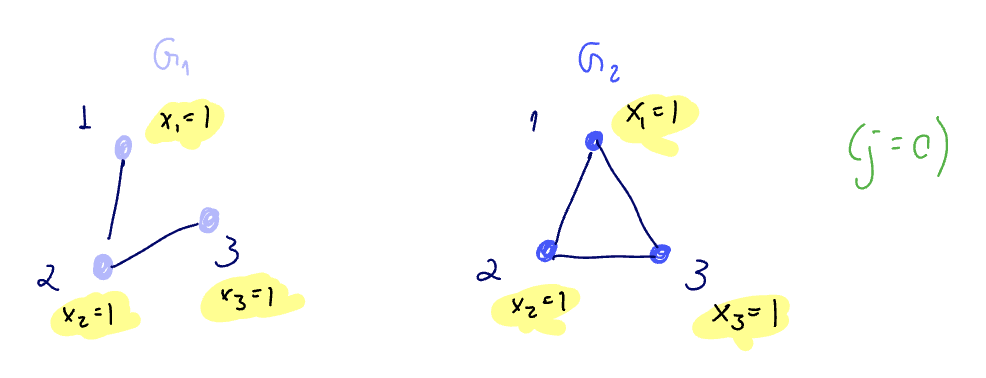
2025-02-24 graphs lecture 10

[[lecture-data]]

Summary

last time

graph isomorphism problem
- GNNs cannot distinguish graphs with identical eigenvalues
- But many non-isomorphic graphs share spectra
- This problem is not solvable in polynomial time
One heuristic is the Weisfeiler-Leman Graph Isomorphism Test

Today

Are GNNs as powerful as the Weisfeiler-Leman Graph Isomorphism Test?
computational graphs
requirements for a powerful GNN
graph isomorphism networks (last architecture we will discuss)

Much of the content from today from
"How Powerful are GNNs" by Xu et al 2019 - created this architecture

measure expressive power wrt WL test

1. Graph Signals and Graph Signal Processing

Recall from last class that we discussed the Weisfeiler-Leman Graph Isomorphism Test, which uses the

Color refinement algorithm

The color refinement algorithm is an algorithm to assign colorings to nodes.

Algorithm

Given graph $G = (V, E)$ with node features $x$

let $c_{i} (0) = f (\cdot, {x_{i}}) \forall i \in V$ (assign colors based on node feature values)
let $t = 0$

while True:

let $c_{i} (t) = f (c_{i} (t - 1), {{c_{j} (t - 1), j \in N (i)}}) \forall i \in V$

assign colors based on previously assigned colors

if $c_{i} (t) == c_{i} (t - 1) \forall i$ , break. else, $t = t + 1$

Here, $f$ is a hash function that assigns colors.

Today, we will finish up the example that we began last class.

Example

Color refinement for

G_{1}

No node features, so assume all 1. First, Assign colors based on node features.

step $t = 0$ :
$c_{1} (0) = c_{2} (0) = c_{3} (0) = f (\cdot, 1) = k_{1}$

step $t = 1$ :
$\begin{aligned} c_{1} (1) & = f (k_{1}, {k_{1}}) & = k_{1} \\ c_{3} (1) & = f (k_{1}, {k_{1}}) & = k_{1} \\ c_{2} (1) & = f (k_{1}, {k_{1}, k_{1}}) & = k_{2} \end{aligned}$
Evaluate: did the colors change?

Yes: continue!

step $t = 2$ :
$\begin{aligned} c_{1} (2) & = f (k_{1}, {k_{1}}) & = k_{1} \\ c_{3} (2) & = f (k_{1}, {k_{1}}) & = k_{1} \\ c_{2} (2) & = f (k_{2}, {k_{1}, k_{1}}) & = k_{2} \end{aligned}$
Evaluate: did the colors change?

No - so we are done!
This is the final coloring.

return ${k_{1}, k_{1}, k_{2}}$

Color refinement for

G_{2}

Again, there are no node features, so we assume the signals are all $1$ .

step $t = 0$ : assign colors based on node features:
$c_{1} (0) = c_{2} (0) = c_{3} (0) = f (\cdot, 1) = k_{1}$
step $t = 1$ :
$\begin{array}{r} c_{1} (1) = c_{2} (1) = c_{3} (1) = f (\cdot, {k_{1}, k_{1}}) = k_{1} \end{array}$

evaluate: did the colors change?

No - so we are done
This is the final coloring

return ${k_{1}, k_{1}, k_{1}}$

Since the outputs of the algorithm are different, we can conclude that $G_{1}$ and $G_{2}$ are not isomorphic.

Note

There are other better algorithms that perform similar tests, but they often come at the expense of more computations

Today, we want to know: Are GNNs as powerful as the Weisfeiler-Leman Graph Isomorphism Test?

Proposition

If a GNN can distinguish between graphs $G_{1}$ and $G_{2}$ , then so can the WL test.

Proof

Consider the $AGGREGATE-COMBINE$ representation of GNNs (recall graph SAGE for something similar) where each layer consists of

aggregation step on the neighborhood of each node

a_{ℓ, i} = AGGREGATE ({(x_{ℓ - 1})_{u} : u \in N (i)})

combine step

(x_{ℓ})_{i} = COMBINE (a_{ℓ, i}, (x_{ℓ - 1})_{i})

And with a permutation invariant readout layer

X_{G} = READOUT ({(x_{ℓ})_{i} : i \in V})

(these are typically like the mean, max, sum, etc)

Suppose after $ℓ$ iterations in the WL test and $ℓ$ layers as described above,

the embeddings $X_{G_{1}} \neq X_{G_{2}}$
the WL test cannot decide if $G_{1}$ and $G_{2}$ are non-isomorphic

If the WL test cannot decide, then every previous iteration $j = 0, 1, \dots, ℓ$ in the test, then

$G_{1}$ and $G_{2}$ must have the same color multisets, call them ${(c_{j})_{v}}$ , and
the color neighborhoods ${(c_{j})_{u} : u \in N (v)}$ are also the same for all $v$

NTS that if WL test for $v \in G_{1}$ and $v^{'} \in G_{2}$ gives the same color, then the GNN gives the same embedding.

want to show

(*)

if the WL test gives $(c_{j})_{v} = (c_{j})_{v^{'}}$ for all $v, v^{'}$ , then the GNN always produces $(x_{j})_{v} = (x_{j})_{v^{'}}$

Since there are no node features, impute $1$ as the feature for all nodes in each graph.

The color refinement algorithm will assign the same colors to all nodes at the initial step as we saw in the example
The 0th layer of the GNN assigns $(x_{0})_{v} = (x_{0})_{v^{'}}$ for all $v, v^{'}$ since all feature values are the same

Induction Hypothesis
Suppose $(*)$ holds for iteration/layer $j$ .

the WL test outputs the same colors $(c_{j + 1})_{v}$ and $(c_{j + 1})_{v^{'}}$ for all $v, v^{'}$ . That is,

[(c_{j})_{v}, {(c_{j})_{u} | u \in N (v)}] = [(c_{j})_{v^{'}}, {(c_{j})_{u^{'}} : u^{'} \in N (v^{'})}]

By the induction hypothesis, we have that

[(x_{j})_{v}, {[x_{j}]_{u} : u \in N (v)}] = [(x_{j})_{v^{'}}, {[x_{j}]_{u^{'}} : u^{'} \in N (v^{'})}]

Since the same $AGGREGATE$ and $COMBINE$ functions are applied to both graphs, then we automatically get that

(x_{j + 1})_{v} = (x_{j + 1})_{v^{'}} \forall v, v^{'}

Thus, by induction, if the colors $(c_{j})_{v} = (c_{j})_{v^{'}}$ for all $v, v^{'}$ , the the embeddings $(x_{j})_{v} = (x_{j})_{v^{'}}$ at any $j$ .

Note

This creates a valid map $(x_{j})_{v} = g ((c_{j})_{v})$ for all $v$ between the embeddings of the nodes and the coloring assignment.

We can extend this mapping to include the multiset of embeddings/colors of the neighbors as well, and say that the multiset of all embeddings and neigeborhood embedding pairs also has a map

{(x_{j})_{v}, {(x_{j})_{u} : u \in N (v)}} = {g ((c_{j})_{v}), {g ((c_{j})_{u}) : u \in N (v)}}

And these are each the same for the two graphs.

Thus, the $(x_{j})_{v}$ and $(x_{j})_{v^{'}}$ are the same for all $j$ . And, due to the permutation invariance of the readout layer as defined above, we must have $X_{G_{1}} = X_{G_{2}}$ .

$⟹ ⟸$ we assumed that the embeddings were NOT equal! Thus, it must be the case that the WL test CAN decide if $G_{1}$ and $G_{2}$ are non-isomorphic.

see the WL test is at least as powerful as a GNN for detecting graph non-isomorphism

What have we shown here?

the WL test is at least as powerful as GNNs

We want to know if GNNs are at least as powerful as the WL test. ie
if the WL test tells $G_{1}$ and $G_{2}$ apart, does there exist a GNN that can tell $G_{1}$ and $G_{2}$ apart?

ie, are GNNs as powerful as the WL test at telling non-isomorphic graphs apart?

Example

Can a GCN tell these apart? Recall

Graph Convolutional Networks

Introduced by Kipf and Willing, 2017, a graph convolutional network layer is given by
$(x_{ℓ})_{i} = σ [\sum_{j \in N (i)} \frac{(x_{ℓ - 1})_{j}}{| N (i) |} H_{ℓ}]$
Note that $H_{ℓ}$ are row vectors. We can think of each layer as a "degree normalized aggregation"

In AGGREGATE-COMBINE form, a GCN layer is given by
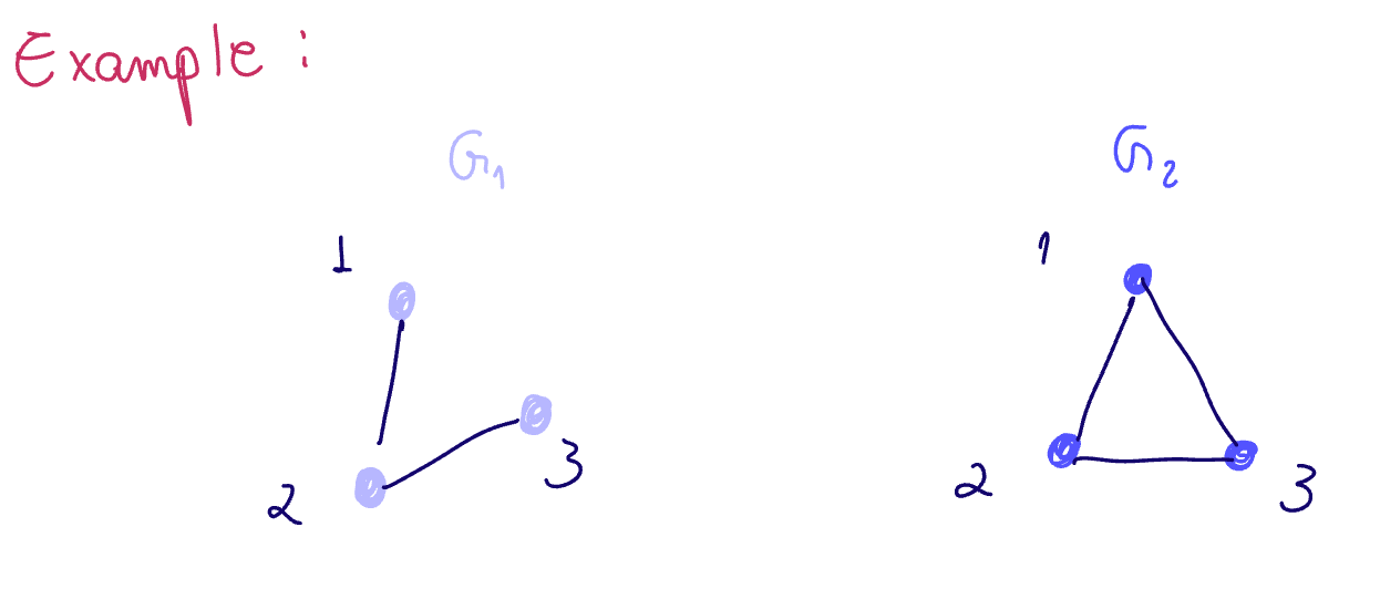
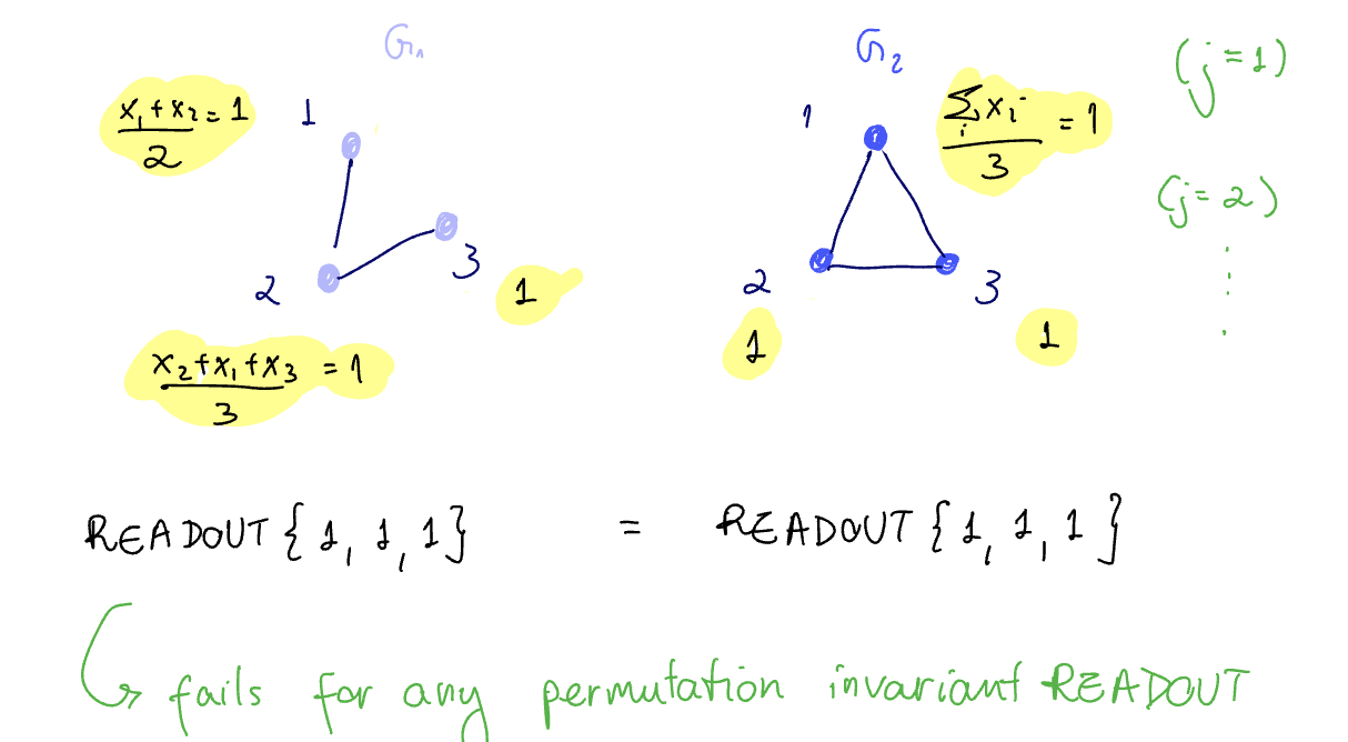
$(x_{j})_{v} = ReLU (W, mean {(x_{j - 1})_{u} : u \in N (v) \cup {}})$
WLOG, assume $W = 1$ . The first layer with readout gives us

But then we get the same output for every layer and this GNN fails for permutation invariant readouts.

Takeaway

By the example above, we can see easily that not every GNN is as powerful as the WL test. However, there are some GNNs that can do better, and which can be at least as powerful.

Exercise

Check if graph SAGE with the $max$ aggregation:

(x_{j})_{v} = max ({ReLU (W . (x_{j})_{u}), \forall u \in N (v)})

Can tell these graphs apart.

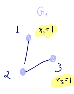
In the example above, where did things break?
Pros: GCNs and any permutation equivariant GNN does not distinguish between nodes 1 and 3. This is an implicit data augmentation mechanism!
Cons: The GCN cannot distinguish between (1 and 3) and 2, but the structure at 1 or 3 is different from at node 2.

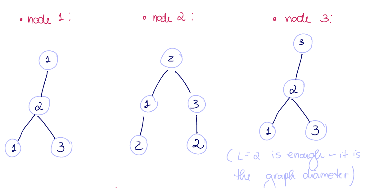
Let's define the computational graph

computational graph

The computational graph tracks the communications that each node makes at each layer or iteration of an algorithm/network.

Example

Since 1 and 3 are symmetric, their computational graph is symmetric

Note

$L = 2$ is sufficient because the diameter (or the longest shortest path between two nodes) is of length 2.

see computational graph

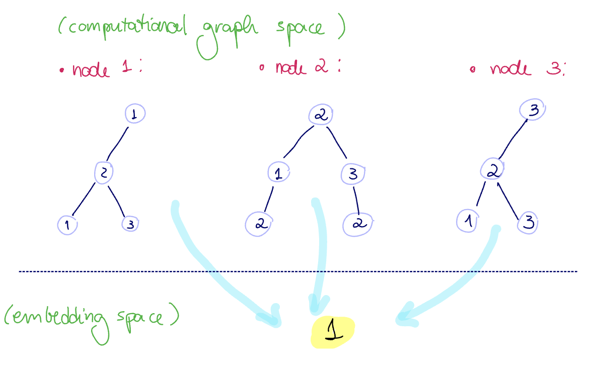
We can imagine that we are mapping computational graphs to some embedding space. The issue with the GCN is that it is mapping all three computational graphs to a single embedding space.

We need functions/embeddings/maps that are injective. ie, which map different computational graphs (or different multisets of embeddings) to different values in embedding space.

Theorem

Let $G_{1}$ and $G_{2}$ be two graphs that the Weisfeiler-Leman Graph Isomorphism Test determines are non-isomorphic. A GNN $Φ$ maps $G_{1}$ and $G_{2}$ to $Φ (G_{1}) \neq Φ (G_{2})$ if the following hold:

$Φ$ aggregates and updates as

(x_{ℓ})_{v} = ϕ ((x_{ℓ - 1})_{v}, φ ({(x_{ℓ - 1})_{u} : u \in N (v)}))

Where $ϕ, φ$ are injective.

The readout function is (permutation invariant) and injective.

Proof (sketch)

In the proof showing that the WL test is at least as powerful as a GNN for detecting graph non-isomorphism, we showed that if the color refinement algorithm gives $(c_{j})_{v} = (c_{j})_{v^{'}} \forall v, v^{'}$ , then the embeddings $(x_{j})_{v} = (x_{j})_{v^{'}} \forall v, v^{'}$ and that that there is a valid map

(x_{j})_{v} = g ((c_{j})_{v}) \forall v

We need $g$ to be injective. Why? We don't want it to be the case that there are different colors $c_{v}, c_{w}$ that map to the same embedding $x_{v}$ .

Let $f$ be the hash function in the WL test. Recall that is is bijective for color multisets. We can write the embedding at layer $j$ as follows:

\begin{aligned} (x_{j})_{v} & = g (f [(c_{j - 1})_{v}, {(c_{j - 1})_{u} : u \in N (v)}]) \\ (x_{j})_{v} & = g (f [g^{- 1} ((x_{j - 1})_{v}), {g^{- 1} ((x_{j - 1})_{u}) : u \in N (v)}]) \\ \approx ϕ (\cdot, φ (\cdot)) the GNN \end{aligned}

So to have $g$ injective, we need the GNN to be injective. Thus,

$ϕ, φ ⟹$ the GNN is injective $⟹ g$ is invective $⟹$ the GNN is as powerful as the WL test

see injective GNNs are as powerful as the WL test