2025-02-19 graphs lecture 9
[[lecture-data]]
2025-02-19
1. Graph Signals and Graph Signal Processing
- This architecture is local because it is still respecting the graph sparsity pattern, and learning the "similarities" of the transformed features at each layer of the network.
- This architecture does not depend on the size of the graph, only the dimension of the features
- It can still be expensive to compute however, if the graph is dense. We need to compute
coefficients , which can be up to in complete graphs.
This additional flexibility increases the capacity of the architecture (less likely to underfit to training data), and this has ben observed empirically. But this comes at the cost of a more expensive forward pass.
This architecture is available and implemented in PyTorch Geometric
We can think of the GAT layer
- however, this architecture is not convolutional since
is changing at each step. - But it can be useful to see how we can write/think about it as something that looks convolutional (if you squint)
the "readout" in graph-level tasks
In graph-level problems, the output does not need to be a graph signal - it could be a scalar, a class label, or some vector in
How do we map GNN layers to such outputs?
We can use "readout" layers
A readout layer is an additional layer added to a GNN to achieve the desired output type/dimension for graph-level tasks or other learning tasks on graphs that require an output that is not a graph signal.
(see readout layer)
In node-level tasks (ex source localization, community detection, citation networks, etc), both the input and the output are graph signals
- Benefit: convolutional graph filters are local. This ensures a parameterization that is independent of graph size
When we learn our GNN layers, we fix
and learn only which does not depend on the graph size.
Option 1
In a fully connected readout layer we define
Where
- in general
vectorizes matrices into vectors
- in general
can be the identity or some other pointwise nonlinearity (ReLU, softmax, etc)
There are some downsides of a fully connected readout layer
- The number of parameters depends on
- adding learning parameters, which grows with the graph size. This is not amenable to groups of large graphs - No longer permutation invariant because of the
operation
Verify that fully connected readout layers are no longer permutation invariant
- No longer transferrable across graphs.
- unlike in GNNs,
depends on . So if the number of nodes changes, we have to relearn
- unlike in GNNs,
These make this a not-so-attractive option, so we usually use an aggregation readout layer
The aggregation readout layer is a readout layer given by
where
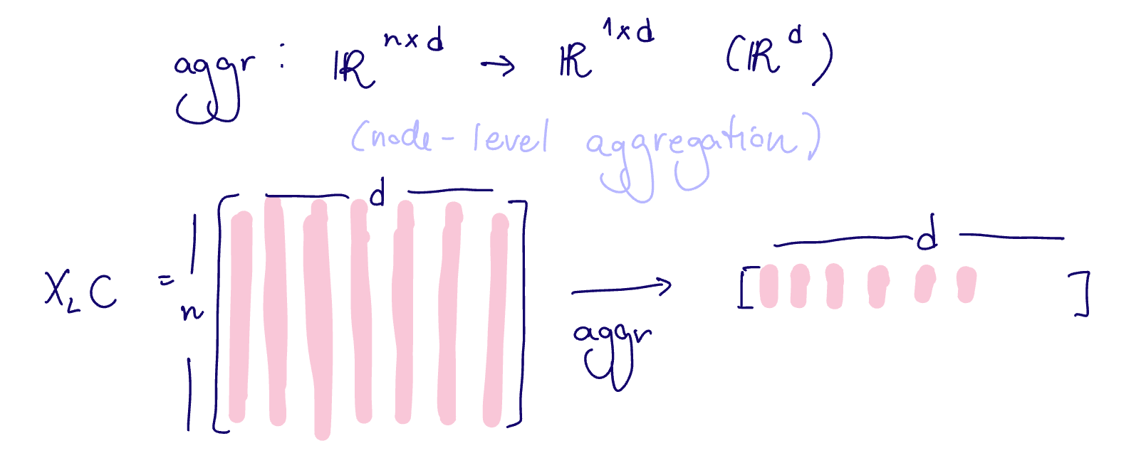
Typical aggregation functions are the mean, sum, max, min, median, etc
- this is now independent of
(my aggregation functions don't change based on the size of my graph) - permutation invariant since the aggregation functions are also permutation invariant
- this remains transferrable across graphs, unlike the fully connected readout layer
graph isomorphism problem
Let
(see graph isomorphism)
A graph isomorphism exists exactly when two graphs are equivalent.
Can we train a GNN to detect if graphs are isomorphic?
- ie, to produce identical outputs for graphs in the same equivalence class/graphs which are isomorphic, and different outputs for graphs that are not isomorphic?
Consider two graphs
- Consider the following single-layer (linear) GNN
Suppose there is some
Consider two graphs
Then there exists a graph convolution we can use to verify whether two graphs are NOT isomorphic, ie to test that
Consider the following single-layer (linear) GNN
Define the graph feature
Set
Then we have
And if there is some
Since the laplacian is positive semidefinite, the sums will be different if and only if we have at least eigenvalue that is different between them.
(see paper GNNs are more powerful than you think)
However, there are many non-isomorphic graphs that share the same eigenvalues
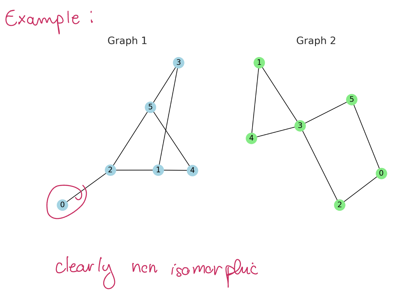
These graphs are clearly non-isomorphic, but their laplacian eigenvalues are the same!
Thus, a strong alternative is the
So our eigenvalue-based heuristic doesn't work for some graphs, but a simple heuristic that does work is counting degrees. Then the problem amounts to comparing the multisets of node degree counts.
(continuing the example from above)
The Weisfeiler-Leman graph isomorphism test consists of running the color refinement algorithm for two graphs.
Since the eigenvalue-based heuristic doesn't work for some graphs, a simple heuristic that does work is counting degrees. Then the problem amounts to comparing the multisets of node degree counts.
The color refinement algorithm is an algorithm to assign colorings to nodes.
Given graph
let
let
while True:
let
- assign colors based on previously assigned colors
if, break.else,
Here,
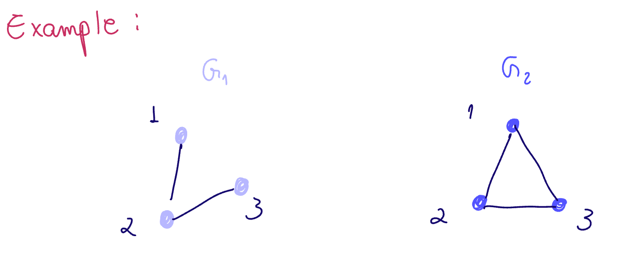
No node features, so assume all 1.
Assign colors based on node features
step
Evaluate: did the colors change?
- Yes: continue!
step
Evaluate: did the colors change?
- No - so we are done!
- This is the final coloring.