2025-02-17 graphs lecture 8
[[lecture-data]]
2025-02-17
coordinate representation and compressed sparse row representation - better explanation of CSR:
If you've taken a numerical LA class, then familiar with seeing how the total # operations is
- information theoretic threshold
- community detection
Today - See [[School/Archived/Equivariant Machine Learning/course_PDFs/Lecture 8.pdf]]
- Popular GNN architectures that can be expressed in convolutional form
- MPNN
- GCN
- ChebNet
- graphSAGE
- GATS
1. Graph Signals and Graph Signal Processing
Recall the definition of a graph neural network:
This is a convolutional GNN because it is based on graph convolution.
- GNNs have great properties which help explain their practical success
This form is general enough to describe a majority of the most popular architectures in use today
Message Passing Neural Network (MPNN)
This type of network was initially introduced by Gilmer et al. In a message passing neural network, each layer consists of 2 operations: the message and the update.
The message is a function that processes
- the signal at node
- the message /signal at each of the neighbors of
- the edge weights
The update is a function on the signal of the graph from the previous layer to the next, taking into account the message and the current value at each node:
Consider an MPNN. As long as
which is a graph convolution with
As long as
Which is a graph convolution with
From the perspective of learning the weights (
Introduced by Kipf and Willing, 2017, a graph convolutional network layer is given by
Note that
We can write a graph convolutional network layer as a graph convolution. This is easy to see by simply writing
Which is exactly the form of a graph convolution with
And A[A>0] in Python)
Advantages of GCNs:
- One local diffusion step per layer
- Simple and interpretable
- Neighborhood size normalization prevents vanishing or exploding gradient problem - only one diffusion step
Disadvantages
- no edge weights
- only supports the adjacency
- No self loops unless they are present in
(embedding at layer not informed by the embedding at layer ). Even if self-loops are in the graph, there is no ability to weight and differently.
The idea behind ChebNets, which were introduced by Defferrard et al. in 2017, in to create a "fast" implementation of graph convolution in the spectral domain. Each layer of a ChebNet is given by
Where
We use the Chebyshev polynomials instead of Taylor polynomials to approximate an analytic function because
- By the chebyshev equioscillation theorem , they provide a better approximation with fewer coefficients
- chebyshev polynomials are orthogonal, meaning we can find an orthonormal basis for free. There is no need to implement the filters in the spectral domain.
(see ChebNet)
Learning in the spectral domain provides an "inductive bias" for learning localized spectral filters
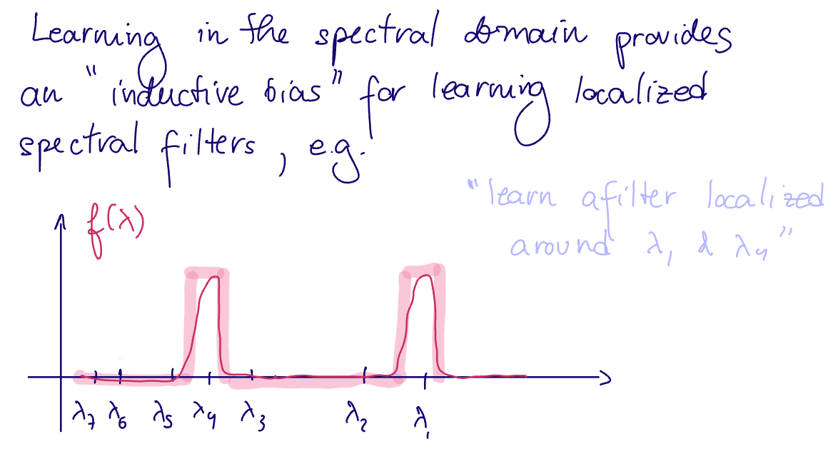
In practice, we need to use an analytic function surrogate for this type of filter (solid red line).
Recall that we can represent any analytic function with convolutional graph filters, but translating back to the spectral domain is expensive because we need to compute the graph fourier transform
This costs 2 additional matrix-vector multiplications, plus the diagonalization of
In the typical spectral representation of a convolutional graph filter, we have
Where
Recall that we can represent any analytic function with convolutional graph filters. Thus, the expressivity of filters is quite strong. However, translating back to the spectral domain is expensive because we need to compute the graph fourier transform
In conventional signal processing, filters based on these polynomials have better cutoff behavior in the spectral domain (compared to general polynomial filters)
- ie, they need fewer coefficients than the Taylor approximation for the same quality
For the formal theorem statement/proof: see chebyshev equioscillation theorem
Using
ie
Intuition why this is better than the Taylor polynomials:
- Chebyshev Polynomial expansion minimizes
norm over the approximation interval ( ), while Taylor series is a local approximation around some
Additionally,
Let
The Chebyshev Polynomials
Advantages
- Fast and cheap - easy to calculate polynomials and they are orthogonal for free
- localized spectral filters
Disadvantages
- less stable than Taylor approximations
- perturbing the adjacency matrix can cause large fluctuations in the chebyshev polynomial approximation, whereas the taylor approximations will remain basically the same
is restricted to - difficult to interpret in the node domain
Introduced by Hamilton-Ying-Leskovee in 2017, each Graph SAGE layer implements the following 2 operations:
Aggregate
Concatenate
The standard
where
(see graph SAGE)
-
SAGE implementations allow for a variety of
functions, including and LSTMs (which look at as a sequence, losing permutation equivariance). In these cases, SAGE is no longer a graph convolution. - There are both advantages and disadvantages of staying a GCN and using other functions.
-
the authors of SAGE popularized the
representation of GNNs (with ) meaning