2025-01-27 graphs lecture 2

Data

subject:: Data Science Methods for Large Scale Graphs

2025-01-27

See [[School/Archived/Equivariant Machine Learning/course_PDFs/Lecture 2.pdf]]

Today

Housekeeping

Scribing sign-up sheet, choose whichever lecture you want by Wednesday
A few lectures cancelled

Last time

[[graph]]s
[[graph signals]]/data with graphs
[[network diffusion process]]/ the way we can process data
general definition of graph diffusion with graph shift operators
- the most common operators were the graph laplacian

Today

interpretation of the [[graph laplacian]]
[[total variation energy]] of graph signals
[[graph frequencies]] and [[oscillation modes]]
the graph fourier transform
graph convolution (maybe)

1. [[Graph Signals and Graph Signal Processing]]

1.1 Interpretation of the (left)/directed [[graph laplacian]]

We begin with an example

Example

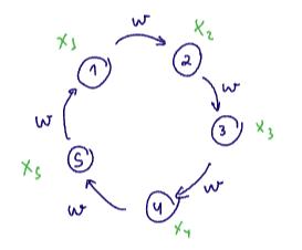
Consider a 5-cycle digraph with some signal $x$ . We can think of this as a periodic signal $x$ sampled at 5 discrete time intervals.

For an $n$ -cycle digraph, we can think of the graph as a periodic signal sampled at $n$ discrete time intervals

Recall the definition of the [[adjacency matrix]]:

Adjacency Matrix

$A_{i j} = {\begin{cases} W (j, i) if (j, i) \in E \\ 0 otherwise \end{cases}$

the adjacency matrix for the 5-cycle digraph is $$A = \begin{bmatrix}
0 & 0 & 0 & 0 & w \
w & 0 & 0 & 0 & 0 \
0 & w & 0 & 0 & 0 \
0 & 0 & w & 0 & 0 \
0 & 0 & 0 & w & 0
\end{bmatrix}$$
The (left) laplacian is

L = D_{out} - A = diag (A 1) - A = [\begin{matrix} w & 0 & 0 & 0 & - w \\ - w & w & 0 & 0 & 0 \\ 0 & - w & w & 0 & 0 \\ 0 & 0 & - w & w & 0 \\ 0 & 0 & 0 & - w & w \end{matrix}]

Let $w = \frac{1}{Δ t}$ . Then $x = [x_{1}, x_{2}, x_{3}, x_{4}, x_{5}]$ is sampled with period $Δ t$ . Let $z = L x$ . Then

z_{i} = {\begin{cases} \frac{1}{Δ t} (x_{i} - x_{i - 1}), z \leq i \leq 5 \\ \frac{1}{Δ t} (x_{1} - x_{5}), i = 5 \end{cases}

Question

What does this definition of $z_{i}$ remind us of?

Answer

This looks like the [[derivative]] of a function $x (t)$ (!!!)

Interpretation of the (left) Graph Laplacian

The [[graph laplacian]] generalizes differentiation to arbitrary graphs.

1.2 Interpretation for the normalized symmetric laplacian

Similar to the [[graph laplacian]], we can build an interpretation for the normalized symmetric laplacian.

Symmetric Laplacian

The symmetric laplacian using the symmetrized adjacency matrix

(see [[symmetric laplacian]])

We will see that the (normalized) [[symmetric laplacian]] generalizes the idea of [[total variation energy]] for [[graph signals]].

Total Variation Energy

The total variation energy of discrete-time signals is defined as

T V (x) = \sum_{i} | x_{i} - x_{i - 1} |

This is a good proxy for the signal frequency (and in fact can be used to estimate it)

Example

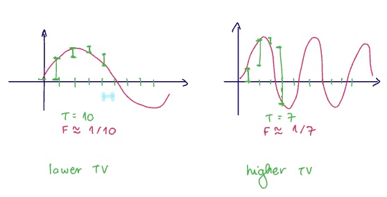
The example on the left with longer period has lower TV. The example on the right with shorter period has higher

High TV -> high frequency
Low TV -> low frequency

1.3 Building to the graph fourier transform 😀

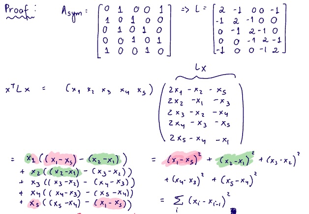
Recall for (now arbitrary) signal on graph $G$ we have $T V (x) = x^{T} L x$ . Suppose $| | x | |_{L} = 1$

Question

What are the lowest and highest values $T V (x)$ can take?

Answer

Let $λ_{1}, λ_{2}, \dots, λ_{n}$ be the eigenvalues of $L$ , ordered by increasing value.

Note that $L 1 = 0$ and $L$ is positive semidefinite $⟹ λ_{1} = 0$ and this is the minimum value for $T V (x)$
The highest value $T V (x)$ can take is $λ_{n}$

Exercise

Show the symmetrized laplacian is positive semidefinite

Important

The TVE gives us a range of values for the frequency of the signal of the graph.

The eigenvalues are the graph's canonical frequencies
the eigenvectors are the oscillation modes of those frequencies.

Tip

From now on, we will assume that the laplacian is the symmetrized version.

Example

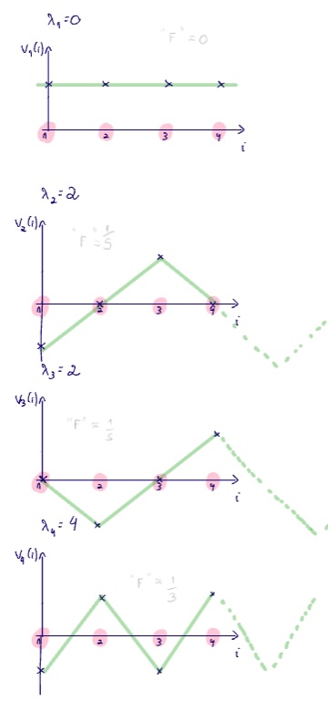
Now, let's consider the 4 digraph. Then

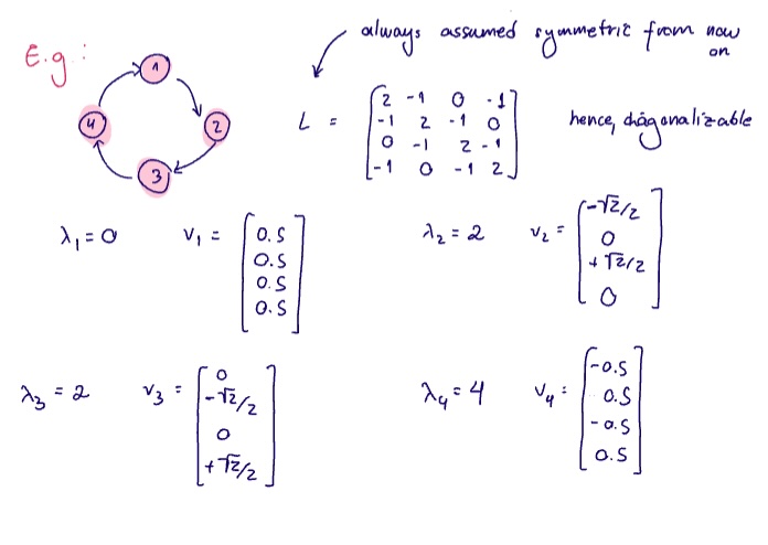
L = [\begin{matrix} 2 & - 1 & 0 & - 1 \\ - 1 & 2 & - 1 & 0 \\ 0 & - 1 & 2 & - 1 \\ - 1 & 0 & - 1 & 2 \end{matrix}]

Since $L$ is symmetric, it is always diagonalizable (see why). As we saw above, $λ_{1} = 0$ and its corresponding eigenvector is $1$ . Thus, the eigenvector will be some multiple of $1$

For the example above,
$λ_{1} = 0, v_{1} = [\frac{1}{2}, \frac{1}{2}, \frac{1}{2}, \frac{1}{2}]$
$λ_{2} = 2, v_{2} = [- \frac{\sqrt{2}}{2}, 0, \frac{\sqrt{2}}{2}, 0]$
$λ_{3} = 2, v_{3} = [0, - \frac{\sqrt{2}}{2}, 0, \frac{\sqrt{2}}{2}]$
$λ_{4} = 4, v_{4} = [- \frac{1}{2}, \frac{1}{2}, - \frac{1}{2}, \frac{1}{2}]$

--- start-multi-column

number of columns: 2  
Shadow: off
Border: on
Column Spacing: 0

We can visualize these vectors as (discrete) time signals, where each of the nodes of the graphs correspond to the sampled locations.

What do we notice?

As the eigenvalue increases, the frequency of the signal increases
$v_{1}$ has frequency $0$
$F (v_{2}) = F (v_{3}) \approx \frac{1}{5}$
$F (v_{4}) \approx \frac{1}{3}$

--- end-column ---

--- end-multi-column

An arbitrary graph is an algebraic extension of a cyclic graph. We can think of a general graph as a discrete sampling of some underlying data manifold.

Notes

Since $L = V Λ V^{T}$ and $V$ is orthogonal, its columns/the eigenvectors (or oscillation modes) form a basis for $R^{n}$

ie, we can represent any graph signal $x$ in this basis

More generally, this is true not just for the laplacian (which is symmetric and thus always diagonalizable), but for any diagonalizable graph shift operator $S$ .

Example

adjacencies of undirected graph
adjacencies of directed graphs, random walk matrix adjacencies and general [[graph laplacian]]s with distinct eigenvalues

(recall that a matrix is diagonalizable if it has all distinct eigenvalues)

Graph Fourier Transform

Given a signal $x$ , the projection of $x$ onto $V$ is called the graph fourier transform of $x$ . ie,

F_{S} (x) = \hat{x} = V^{*} x, \hat{x} \in R^{n}

and ${\hat{x}}_{i} = v_{i}^{*} x_{i} = ⟨ v_{i}, x ⟩$ (where $v_{i}$ is the $i$ th column of $V$ )

(see [[graph fourier transform]])

Example

Back to our 5 cycle example. Let's define a diagonalizable operator as follows:

The eigenvalues are the complex exponentials $λ_{j} = \exp {- i \frac{2 π}{5} (j - 1)}$
The eigenvectors are given by the fourier basis, ie $V$ is given by

V_{j k} = \exp {- i \frac{2 π}{5} (j - 1) \cdot (k - 1)}

The GFT here is then
${\hat{x}}_{k} = \frac{1}{\sqrt{5}} \sum_{n = 0}^{4} x_{n + 1} \exp {- i \frac{2 π}{5} (n \cdot k)}$
And for general cyclical graphs on $N$ nodes:
${\hat{x}}_{k} = \frac{1}{\sqrt{N}} \sum_{n = 0}^{N - 1} x_{n + 1} \exp {- i \frac{2 π}{N} (n \cdot k)}$
And this is precisely the definition of the discrete Fourier transform(!!) ie, we can recover the classical definition for the (discrete) Fourier transform using our definition for the graph version.

Main Takeaway

The Fourier Transform in euclidian space into graph signal space.

Notes

In general, the interpretation of the adjacency eigenvalues as graph frequencies is not as clean as it is for the laplacian.
- The eigenvectors of $A$ and $L$ do not generally match, and there is no alternative definition in terms of $A$ .
In practice, it is generally true that low-magnitude adjacency eigenvalues correspond to high graph frequencies and vice versa.
When considering the normalized adjacency matrix and the normalized laplacian, it is easy to see that the eigenvectors are the same.
- But in this case, the adjacency eigenvalues can NOT be interpreted as graph frequencies.